Efficient Filtering and Fitting of Models Derived from Integro-Difference Equations
1 Introduction
The Integro-Difference equation model (here abbreviated as IDEM or IDE 1) is a dynamics-based spatio-temporal aiming to model diffusion and convection by making the value of a process a weighted average of it’s previous time, plus noise.
As common and widespread as the problem is, spatio-temporal modelling still presents a great deal of difficulty. Inherently, spatio-temporal datasets are almost always high-dimensional, especially when considering image data (where each pixel might be considered an observation). Additionally, repeated observations are usually not possible due to their time dependence.
Traditionally, the problem has been tackled by the moments (usually the means and covariances) of the process in order to make inference (Wikle et al. (2019), for example, call this ‘descriptive’ modelling). While this method can be sufficient for many problems, there are many cases where we are underutilizing some knowledge of the underlying dynamic systems involved. For instance, in temperature models, we know that temperature has movement (convection) and spread (diffusion), and that the state at any given time will depend on its state at previous times 2. We call models which make use of this ‘dynamic’ models.
2 Integro-difference Based Dynamics
A general way of writing a hierarchical (discrete-time) dynamical model might be
\[\begin{split} Y_{t+1}(\cdot) &= \mathcal M_t(Y_0(\cdot), \dots, Y_t(\cdot)) + \nu_t(\cdot), \quad t=0, \dots, T-1,\\ Z_t(\cdot) &= \mathcal O_t(Y_t(\cdot)) + x(\cdot)^{\intercal}\bm \beta + \epsilon_t(\cdot), \quad t=1,\dots,T. \end{split} \]
This describes the scalar random fields \(Z_t(\cdot), Y_t(\cdot)\in \mathbb R\) over the space \(\mathcal D\subset \mathcal R^d\), which are the observed data and unobserved dynamic process, respectively. \(\mathcal M_t\) here is a non-random ‘propagation operator’, defining how the process evolves with respect to it’s previous state(s), and \(\mathcal O_t\) is a non-random ‘observation operator’, defining how observations of a given process state are taken. Both these fields have random (usually time-independent) additive random fields, \(\nu_t(\cdot), \epsilon_t(\cdot)\), and we also include non-random measured linear covariate terms \(x(\cdot)^{\intercal}\bm \beta\).
If we discretize the space into \(n\) spatial locations \(\{\bm s_i\}_{i=1,\dots, n}\), assume the operators are linear, assert a Markov condition, and assume the errors are all normal, we get a simple linear dynamic system;
\[\begin{split} \bm Y_{t+1} &= M_t\bm Y_t + \bm \nu_t, \quad t=0, \dots, T-1,\\ \tilde{\bm Z}_t &= O_t\bm Y_t + \bm \epsilon_t, \quad t=1,\dots,T, \end{split} \tag{1}\]
where we have written \(\bm Y_t = (Y_t(\bm s_1),\dots, Y_t(\bm s_n))\), and similar for \(\bm Z_t, \bm \epsilon_t\) and \(\bm\nu_t\), and we have written \(\tilde{\bm Z}_t = \bm Z_t + X^{\intercal}\bm \beta\). This is a well-known type of system, the process \(Y\) can easily be estimated either directly of with a Kalman filter/smoother and variants, which will be discussed later.
However, this model is restrictive and high-dimensional; \(M_t\), the primary quantities which need estimation, is of dimension \(n\times n\), of which there are \(T\) matrices to be estimated. Even if we allow the propagation matrix to be invariant in time, we can still only make predictions at the stations \(\{\bm s_i\}\).
This motivates a different approach; in particular, one which allows us to estimate the random field at arbitrary points \(Y_t(\bm s)\) using some spectral decomposition, which would alleviate these problems.
The Integro-difference equation model attempts to generalise Equation 1 into the continuous space by replacing the discrete linear \(M_t\) by a continuous integral equivalent;
\[\begin{split} Y_{t+1}(\bm s) &= \int_{\mathcal D_s} \kappa_t(\bm s,\bm r) Y_t(\bm r) d\bm r + \nu_t(\bm s), \quad t=0, \dots, T-1, \\ Z_t(\bm s) &= Y_t(\bm s) + X(\bm s)^{\intercal}\bm \beta + \epsilon_t(\bm s), \quad t=1,\dots,T. \end{split} \tag{2}\]
Where \(\nu_t(\bm s)\) is a small scale gaussian variation with no temporal dynamics (Cressie and Wikle 2015 call this a ‘spatially descriptive’ component), \(\bm X(\bm s)\) are spatially varying covariates (for example, in a large-scale climate scenario, this might be latitude, concentration of some chemical/element like nitrogen) \(\kappa(\bm s, \bm r)\) is the driving ‘kernel’ function, and \(\epsilon_t\) is a Gaussian white noise ‘measurement error’ term.
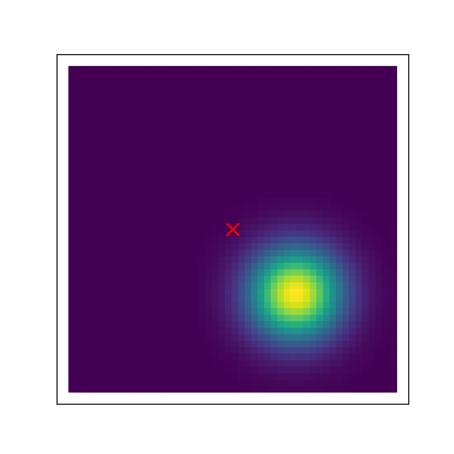
Our operator is now \(\mathcal M(Y_t(\bm s)) = \int_{\mathcal D_s} \kappa_t(\bm s,\bm r) Y_t(\bm r) d\bm r\), which can model diffusion and convection by choosing the shape of \(\kappa\) (which, from now on, we will assume to be temporally invariant). This kernel defines how each point in space is affected by every other point in space at the previous time. For example, if we choose a Gaussian-like shape,
\[\begin{split} \kappa(\bm s, \bm r; \bm\theta_\kappa(\bm s)) = \frac{\gamma}{2\pi\delta}\exp\left(-\frac{1}{2\delta^2}\|\bm r - \bm s - \bm\tau(\bm s)\|^2\right), \end{split} \]
then the ‘flow’ would be in the direction of \(\bm\tau(\bm s)\), the diffusion controlled by \(\delta\), and the decay by \(\gamma\). This creates a ‘spatially variant kernel’, where the direction of flow varies across the space, as illustrated in Figure 1.

3 Spectral Representations
We work in the spectral domain of the process, as in Wikle and Cressie (1999) in order to coerce the model hierarchy into a more familiar linear dynamical system form, like Equation 1.
This kind of dimension-reduction allows us to parametrise spatial fields with as few or as many parameters as we want.
3.1 Process decomposition
Choose a complete class of spatial spectral basis functions, \(\{\phi_i(\cdot): \mathcal D\to \mathbb R\}_{i=1,\dots}\), and decompose the process spatial field at each time;
\[\begin{split} Y_t(\bm s) \approx \sum_{i=1}^{r} \alpha_{i,t} \phi_i(\bm s), \quad t=0,\dots,T. \end{split} \tag{3}\]
where we truncate the expansion at some \(r\in\mathbb N\). Notice that we can write this in vector/matrix form, where we consider the vector field \(\bm \phi(\cdot) = (\phi_1(\cdot),\dots, \phi_r(\cdot))^\intercal\); considering times \(t=1,2,\dots, T\), we set
\[\begin{split} \bm \phi(\bm s) &= (\phi_1(\bm s), \phi_2(\bm s), \dots, \phi_r(\bm s))^{\intercal},\\ \bm \alpha_t &= (\alpha_{1,t}, \alpha_{2,t}, \dots, \alpha_{r, t})^{\intercal}. \end{split} \tag{4}\]
Now, (Equation 3) gives us, for any \(\bm s\in \mathcal D\),
\[\begin{split} Y(\bm s; t) \approx \bm \phi^{\intercal}(\bm s) \alpha(t).\\ \end{split} \tag{5}\]
We can effectively now work exclusively with \(\bm \alpha_t = (\alpha_{1,t},\dots, \alpha_{r,t})^\intercal\). To do so, we need to find the evolution equation of \(\bm \alpha_t\), as given below.
Theorem 1 (Spectral form of the state evolution) Define the Gram matrix;
\[\Psi \coloneq \int_{\mathcal D_s} \bm \phi(\bm s) \bm \phi(\bm s)^\intercal d\bm s. \tag{6}\]
Then, the basis coefficients evolve by the equation
\[\bm \alpha_{t+1} = M \bm\alpha_t + \bm\eta_t, \tag{7}\]
where \(M = \Psi^{-1} \int\int \bm\phi(\bm s) \kappa(\bm s, \bm r)\bm\phi(\bm r)^\intercal d\bm r d \bm s\) and \(\bm\eta_t =\Psi^{-1} \int \bm \phi(\bm s)\nu_t(s)d\bm s\).
Proof. (Adapting from Dewar et al. 2008), write out the process equation, (Equation 2), using the first equation of (Equation 5);
\[Y_{t+1}(\bm s) = \bm \phi(\bm s)^{\intercal} \alpha_{t+1} = \int_{\mathcal D_s} \kappa(\bm s, \bm r) \bm\phi(\bm r)^{\intercal}\bm \alpha_t d\bm r + \nu_t(\bm s), \]
We then multiply both sides by \(\bm \phi(s)\) and integrate over \(\bm s\)
\[\begin{split} \int_{\mathcal D_s} \bm\phi(\bm s)\bm\phi(\bm s)^{\intercal} d\bm s \bm\alpha_{t+1} &= \int\bm\phi(\bm s)\int \kappa(\bm s, \bm r)\bm\phi(\bm r)^\intercal d\bm r d \bm s\ \bm\alpha_t + \int \bm \phi(\bm s)\nu_t(s)d\bm s\\ \Psi \bm\alpha_{t+1} &= \int\int \bm\phi(\bm s)\kappa(\bm s, \bm r) \bm\phi(\bm r)^\intercal d\bm r d \bm s\ \bm\alpha_t + \int \bm \phi(\bm s)\nu_t(s)d\bm s. \end{split} \]
So, finally, pre-multipling by the inverse of the gram matrix, \(\Psi^{-1}\) (Equation 6), we arrive at the result.
3.2 Spectral form of the Process Noise
We still have to set out what the process noise, \(\nu_t(\bm s)\), and its spectral counterpart, \(\bm \eta_t\), are. Dewar et al. (2008) fix the variance of \(\nu_t(\bm s)\) to be uniform and uncorrelated across space and time, with \(\nu_t(\bm s) \sim \mathcal N(0,\sigma^2)\) It is then easily shown that \(\bm\eta_t\) is also normal, with \(\bm\eta_t \sim \mathcal N(0, \sigma^2\Psi^{-1})\).
However, in practice, we simulate in the spectral domain; that is, if we want to keep things simple, it would make sense to specify (and fit) the distribution of \(\bm\eta_t\), and compute the variance of \(\nu_t(\bm s)\) if needed.
Lemma 1 Let \(\bm\eta_t \sim \mathcal N(0, \Sigma_\eta)\), and \(\cov[\bm\eta_t, \bm \eta_{t+\tau}] =0\), \(\forall \tau>0\). Then \(\nu_t(\bm s)\) has covariance
\[\cov [\nu_t(\bm s), \nu_{t+\tau}(\bm r)] = \begin{cases} \bm\phi(\bm s)^\intercal \Sigma_\eta \bm\phi(\bm r) & \text{if }\tau=0\\ 0 & \text{else.}\\ \end{cases} \]
Proof. Consider \(\Psi \bm\eta_t\), and consider the case \(\tau=0\). It is clearly normal, with zero expectation and variance (using Equation 6),
\[\begin{split} \var[\Psi \bm\eta_t] &= \Psi \var[\bm\eta_t] \Psi^\intercal = \Psi\Sigma_\eta\Psi^\intercal,\\ &= \int_{\mathcal D_s} \bm\phi(\bm s) \bm\phi(\bm s)^\intercal d\bm s \ \Sigma_\eta \ \int_{\mathcal D_s} \bm\phi(\bm r) \bm\phi(\bm r)^\intercal d\bm r\\ &= \int\int_{\mathcal D_s^2} \bm\phi(\bm s) \bm\phi(\bm s)^\intercal \ \Sigma_\eta \ \bm\phi(\bm r) \bm\phi(\bm r)^\intercal d\bm r d\bm s\\ \end{split} \tag{8}\]
Since it has zero expectation, we also have
\[\begin{split} \var[\Psi\bm\eta_t] &= \mathbb E[(\Psi\bm\eta_t) (\Psi\bm\eta_t)^\intercal] = \mathbb E[\Psi\bm\eta_t\bm\eta_t^\intercal\Psi^\intercal]\\ &= \mathbb E \left[ \int_{\mathcal D_s} \bm\phi(\bm s)\nu_t(\bm s)d\bm s \int_{\mathcal D_s} \bm \phi(\bm r)^\intercal \nu_t(\bm r) d\bm r \right]\\ &= \int\int_{\mathcal D_s^2} \bm\phi(\bm s)\ \mathbb E[\nu_t(\bm s)\nu_t(\bm r)]\ \bm \phi(\bm r)^\intercal d\bm s d \bm r. \end{split} \tag{9}\]
We can see that, comparing (Equation 8) and (Equation 9), we have
\[\cov [\nu_t(\bm s), \nu_t(\bm r)] = \mathbb E[\nu_t(\bm s)\nu_t(\bm r)]= \bm\phi(\bm s)^\intercal \Sigma_\eta \bm\phi(\bm r). \]
Since, once again, \(\mathbb E[\bm\nu_t(\bm s)]=0\).
For the \(\tau\neq0\) case, it is simple to show that the covariance is 0.
3.3 Kernel Parameterisations
Next is the part of the system, which defines the dynamics; the kernel function, \(\kappa\). There are a few ways to handle the kernel. One of the most obvious is to expand it out into a spectral decomposition as well;
\[\kappa \approx \sum_i \beta_i\psi(\bm s, \bm r). \]
This can allow for a wide range of interestingly shaped kernel functions, but see how these basis functions must now act on \(\mathbb R^2\times \mathbb R^2\); to get a wide enough space of possible functions, we would likely need many terms in the spectral expansion.
A much simpler approach would be to simply parametrise the kernel function, to \(\kappa(\bm s, \bm r, \bm \theta_\kappa)\). We then establish a simple shape for the kernel (e.g. Gaussian) and rely on very few parameters (for example, scale, shape, offsets). The example kernel used in the jaxidem is a Gaussian-shape kernel;
\[\kappa(\bm s, \bm r;\, \bm\theta_\kappa) = \frac{\gamma}{2\pi\delta^2}\exp\!\left(-\frac{\|\bm r - \bm s - \bm\tau\|^2}{2\delta}\right), \]
where \(\gamma\) is a decay parameter, \(\delta\) controls the bandwidth, and \(\bm\tau\) is a constant offset. Of course, this kernel lacks spatial dependence. We can add spatial variance back by adding dependence on \(\bm s\) to the parameters, for example, varying the offset term as \(\bm\tau(\bm s)\). Of course, now we are back to having entire functions as parameters, but taking the spectral decomposition of the parameters we actually want to be spatially variant seems like a reasonable middle ground (Cressie and Wikle 2015). The actual parameters of such a spatially-variant kernel are then the spectral coefficients for the expansion of any spatially variant parameters, as well as any constant parameters. This is precisely what is plotting in Figure 1, where the spectral coefficients are randomly sampled from a multivariate normal distribution;
\[\begin{split} \bm\tau(\bm s) = \left(\begin{matrix} \sum_{i=1}^{r_\tau} \psi_{\kappa,i}(\bm s)\, \tau_{1,i}\\ \sum_{i=1}^{r_\tau} \psi_{\kappa,i}(\bm s)\, \tau_{2,i} \end{matrix}\right), \end{split} \]
where \(\tau_{1,i}\) and \(\tau_{2,i}\) are coefficients for the x and y coordinates respectively, and \(\psi_{\kappa, i}(\bm s)\) are basis functions (using cosine or Fourier basis funcitons reveals a convenient formula to significantly simplify the computation of the matrix \(M\)).).
3.4 IDEM as a linear dynamical system
To summarise, we have taken a truncated spectral decomposition to write the Integro-difference equation model as a more traditional linear dynamical system form (Equation 7). All that is left is to include our observations in our system.
Lets assume that at each time \(t\) there are \(n_t\) observations at locations \(\bm s_{1,t},\dots, \bm s_{n_{t},t}\). We write the vector of the process at these points as \(\bm Y(t) = (Y(s_{1,t};t), \dots, Y(s_{n_{t},t};t))^\intercal\), and, in it’s expanded form \(\bm Y_t = \Phi_t \bm\alpha_t\), where \(\Phi \in \mathbb R^{r\times n_{t}}\) is
\[\begin{split} \{\Phi_{t}\}_{i, j} = \phi_{i}(s_{j,t}). \end{split} \]
For the covariates, we write the matrix \(X_t = (\bm X(\bm s_{1, t}), \dots, \bm X(\bm s_{1=n_{t}, t})^\intercal\). We then have
\[\begin{split} \bm Z_t &= \Phi \bm \alpha_t + X_{t} \bm \beta + \bm \epsilon_t, \quad t = 1,\dots, T,\\ \bm \alpha_{t+1} &= M\bm \alpha_t + \bm\eta_t,\quad t = 0,1,\dots, T-1,\\ M &= \left[\int_{\mathcal D_s}\bm\phi(\bm s) \bm\phi(\bm s)^\intercal d\bm s\right]^{-1} \int_{\mathcal D_s^2}\bm\phi(\bm s) \kappa(\bm s, \bm r; \bm\theta_\kappa)\bm\phi(\bm r)^\intercal d\bm r d \bm s, \end{split} \]
Writing \(\tilde{\bm{Z}}_t = \bm Z_t - X_t \bm \beta\),
\[\begin{split} \tilde{\bm Z}_t &= \Phi_{t} \bm \alpha_t + \bm \epsilon_t,\quad &t = 1,2,\dots, T,\\ \bm \alpha_{t+1} &= M \bm \alpha_t + \bm\eta_t,\quad &t = 0,1, \dots, T-1.\\ \end{split} \tag{10}\]
We should also initialise \(\bm \alpha_0 \sim \mathcal N^{r}(\bm m_{0}, \Sigma_{0})\), and fix simple distributions to the noise terms,
\[\begin{split} \bm \epsilon_{t} \overset{\mathrm{iid}}{\sim} \mathcal N_{n_\mathrm{obs}}(0,\Sigma_\epsilon),\\ \bm \eta_{t} \overset{\mathrm{iid}}{\sim} \mathcal N_{R}(0,\Sigma_\eta), \end{split} \]
which are independent in time.
As in, for example, (Wikle and Cressie 1999), Equation 10 is now in a traditional enough form that the Kalman filter can be applied to filter and compute many necessary quantities for inference, including the marginal likelihood. We can use these quantities for maximum likelihood estimation, EM algorithm maximisation, or a Bayesian approach; these will be discussed in an upcoming paper.
References
Footnotes
Historically, this has been abbreviated as IDE. However, with that abbreviation almost universally meaning ‘Integrated Development Environment’, here, we often choose to include the ‘M’ in the abbreviation.↩︎
at least, in a discrete-time scenario. Integro-difference based mechanics can be derived from continuous-time convection-diffusion processes, see Liu et al. (2022)↩︎